
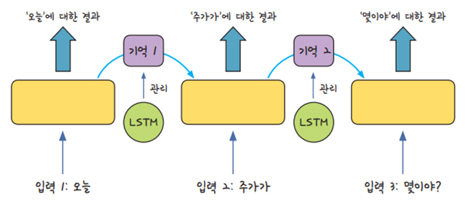
- 여러 개의 데이터가 순서대로 입력되었을 때 앞서 입력 받은 데이터를 잠시 기억함
- 기억된 데이터가 얼마나 중요한지 판단하고 별도의 가중치를 주어 다음 데이터로 넘어감
- 모든 입력에 이 작업을 순서대로 실행하므로 다음 층으로 넘어가기 전에 같은 층을 맴도는 것처럼 보임
LSTM(Long Short Term Memory)
- 한 층 내에서 반복을 많이 해야 하는 RNN의 특성상 일반 신경망보도 ‘기울기 소실 문제’가 더 많이 발생하고 이를 해결하기 어려움. 이러한 단점을 보완하기 위해 등장한 기법
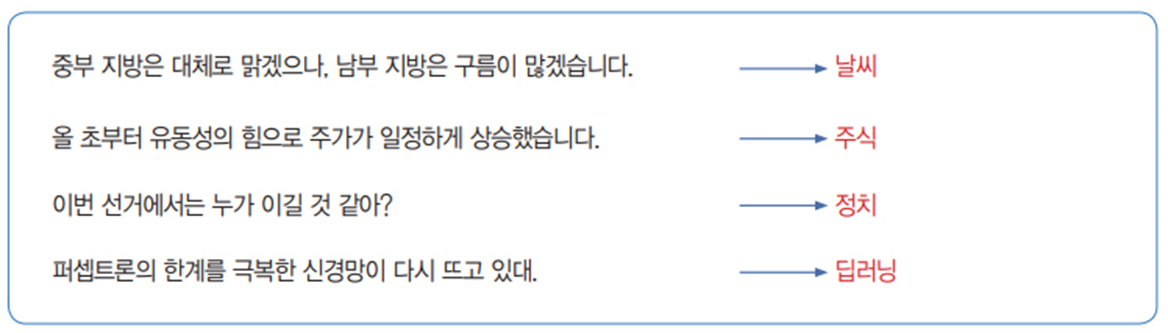
LSTM을 이용한 로이터 뉴스 카테고리 분류
데이터 불러오기
from tensorflow.keras.datasets import reuters

(X_train, y_train),(X_test, y_test) = \
                      reuters.load_data(num_words=None, test_split=0.2)
데이터 확인
print( type(X_train) )                      # 학습 데이터 셋의 데이터 형 확인
print( X_train.shape )                      # 학습 데이터 셋의 크기 확인
print('학습용 뉴스 기사 개수 :', len(X_train))  # 8982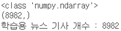
import numpy as np
print('카테고리를 표현한 가장 작은 수 :', np.min(y_train))
print('카테고리를 표현한 가장 큰 수 :', np.max(y_train))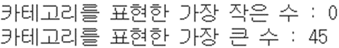
categroy = np.max(y_train) + 1                  # 카테고리 수(클래수 수) : 46
print('카테고리 수 :', categroy)print( X_train[0] )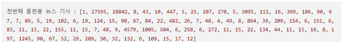
print( len(X_train[0]) ) # 87length_samples = [len(sample) for sample in X_train ]
print('뉴스 기사 데이터(샘플)의')
print('최대 길이 :', max(length_samples))
print('평균 길이 :', np.mean(length_samples))
print('최소 길이 :', min(length_samples))
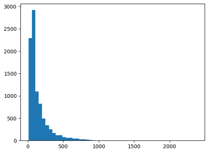
import matplotlib.pyplot as plt
plt.hist(length_samples, bins = 50)
plt.show()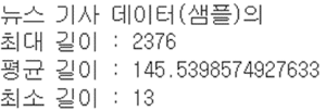
word_to_index = reuters.get_word_index()
print(len(word_to_index))
print(word_to_index)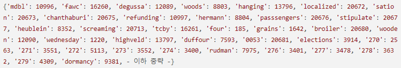
index_to_word = {}
for key, value in word_to_index.items():
  index_to_word[value] = key

index_to_word[1]  # 'the'

index_to_word[128]   #  'tax'
for index, token in enumerate( ('<pad>', '<sos>', '<unk>')):
  print(index, token)
  index_to_word[index] = token
' '.join( [index_to_word[index] for index in X_train[0]] )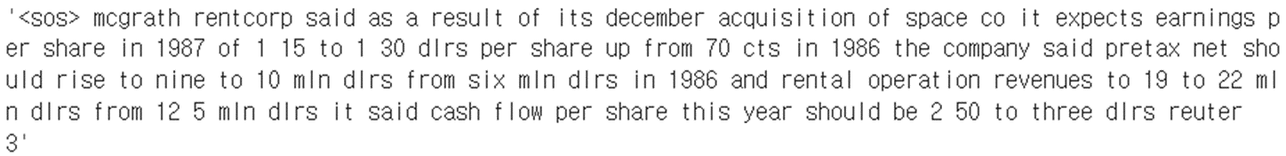
print('테스트용 뉴스 기사 개수 :', len(X_test)) # 2246
print(len(X_train[0]), X_train[0] ) # 학습 데이터 셋의 첫 번째 입력 값 확인-87 [1, 27595, 28842, 8, 43, 10, 447, … ]
- Load_data(num_words=None, test_split=0.2)에서 num_words의 의미
- 매개변수 num_words = 1000이라고 설정하면 단어의 등장 빈도가 1부터 1000만 입력 데이터로 사용하라는 뜻
from tensorflow.keras.datasets import reuters
import numpy as np
from tensorflow.keras.utils import to_categorical
from tensorflow.keras.callbacks import EarlyStopping
from tensorflow.keras.preprocessing import sequence
from tensorflow.keras.models import Sequential
from tensorflow.keras.layers import Dense, LSTM, Embedding

# 학습셋과 데이터셋으로 나누기
(X_train, y_train),(X_test, y_test) = \
                      reuters.load_data(num_words = 1000, test_split=0.2)

# 카테고리 수(클래수 수) : 46
categroy = np.max(y_train) + 1

print( X_train[0] )  # [1, 2, 2, 8, 43, 10, …]

# 학습 데이터 셋의 각 샘플의 요소의 개수가 같도록 맞춤
X_train = sequence.pad_sequences(X_train, maxlen=100)
X_test = sequence.pad_sequences(X_test, maxlen=100)

from tensorflow.keras.utils import to_categorical
y_train = to_categorical(y_train)
y_test  = to_categorical(y_test)

# 모델 구조 설정
model = Sequential()

model.add(Embedding(1000,100))
model.add(LSTM(100, activation='tanh'))
model.add(Dense(46, activation='softmax'))

# 모델의 실행 옵션을 정합니다.
model.compile(loss='categorical_crossentropy', optimizer='adam', \
              metrics=['accuracy'])

# 학습 조기 중단을 설정합니다.
early_stopping_callback = EarlyStopping(monitor='val_loss', patience=5)

# 모델을 실행합니다.
history = model.fit(X_train, y_train, batch_size=20, epochs=200, \
                    validation_data=(X_test, y_test),\
                    callbacks=[early_stopping_callback])
print('\n Test Accuracy: %.4f' % (model.evaluate(X_test, y_test)[1]))
import matplotlib.pyplot as plt

# 학습셋과 테스트셋의 오차를 저장합니다.
y_vloss = history.history['val_loss']
y_loss = history.history['loss']

# 그래프로 표현해 보겠습니다.
x_len = np.arange(1, len(y_loss)+1)
plt.plot(x_len, y_vloss, marker='.', c="red", label='Validset_loss')
plt.plot(x_len, y_loss, marker='.', c="blue", label='Trainset_loss')

# 그래프에 그리드를 주고 레이블을 표시하겠습니다.
plt.legend(loc='upper right')
plt.grid()
plt.xlabel('epoch')
plt.ylabel('loss')
plt.xlim([1, len(y_loss)+1])
plt.show()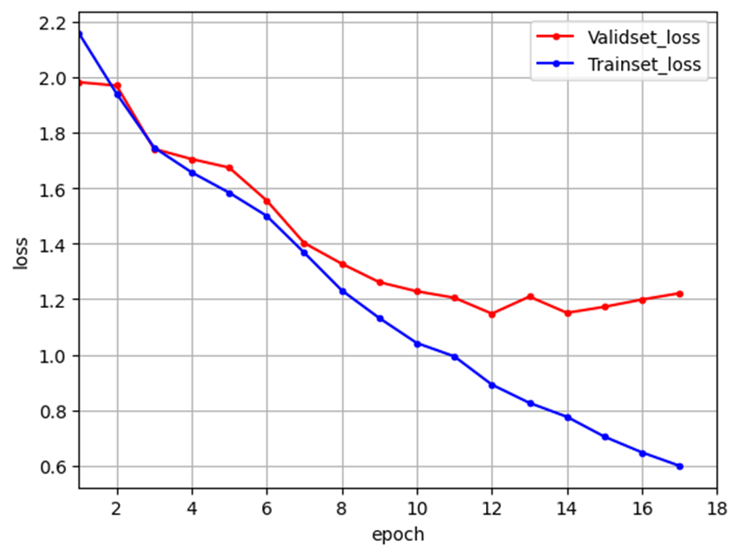
'빅데이터 분석가 양성과정 > Python - 딥러닝' 카테고리의 다른 글
| DNN을 이용한 영상 분류_재정리 (0) | 2024.07.18 |
|---|---|
| 딥러닝 사전지식 ( Pre-knowledge ) (1) | 2024.07.17 |
| 딥러닝을 이용한 자연어 처리 (1) | 2024.07.17 |
| 이미지 인식 - CNN (0) | 2024.07.17 |
| 실습 (0) | 2024.07.17 |